Eric Bannatyne

This post is based on an advanced tutorial for CSC373: Algorithm Design, Analysis, and Complexity, which I presented on January 30, 2017. For more information, check out the course textbook [2], and [3].

If you’ve ever done anything involving signal processing or data analysis, there’s a good chance that you’ve heard of the fast Fourier transform. Originally explored to solve some specific engineering problems, and first published in its general form—as we know it today—by James Cooley and John Tukey in 1965 [1], the fast Fourier transform is an incredibly famous algorithm that has tons of applications in areas like digital signal processing, speech recognition, data compression, communications, and computer vision, to name a few.

The goal of this post is to introduce the fast Fourier transform, by looking specifically at how it can be applied to obtain efficient algorithms for polynomial multiplication.

Polynomial Multiplication

Suppose that we are given two polynomials of degree n−1:¹

A(x)=a0+a1x+a2x2+⋯+an−1xn−1B(x)=b0+b1x+b2x2+⋯+bn−1xn−1.

We wish to find the product of A and B, a polynomial C such that C(x)=A(x)B(x). Suppose that we represent A as a vector of its n coefficients a=(a0,…,an−1), and likewise B with b=(b0,…,bn−1). Then there is a straightforward algorithm for computing the coefficients of C, by simply expanding out the algebraic expression A(x)B(x) and collecting like terms—essentially what you would have done in your high school algebra class. This procedure takes Θ(n2) operations, since we’re essentially multiplying all pairs of coefficients from A and B. In the rest of this post, we’ll derive a faster method of computing the product C.

As an aside, the algorithm for polynomial multiplication that we’re about to discover also forms the basis for what were, until recently, some of the best-known algorithms for integer multiplication. If you think about it a bit, this should make some intuitive sense: You can think of the coefficients (a0,…,an−1) as representing the digits of an integer in a given base (typically base 2), when this base is substituted for the variable x. Then integer multiplication is kind of like polynomial multiplication, except that we also have to take into account carry digits. Combining the fast Fourier transform with several clever number theory tricks gives us the Schönhage–Strassen algorithm, which lets us multiply two n-digit integers in time O(nlognloglogn).

Representing Polynomials

So far, we’ve assumed that a polynomial is represented by its list of coefficients. However, the following fact will suggest an alternative way of representing polynomials.

Fact. A set of n point-value pairs (say in R2 or C2) uniquely determines a polynomial of degree n−1.

This is essentially a generalization of the statement “given two points in the plane, there is a unique line that passes through them.” Proving this is an exercise in linear algebra; given n point-value pairs, we can compute the coefficients of a polynomial passing through those points by solving a system of linear equations.²

This leads us to the point-value representation of a polynomial: Given points x0,…,xn−1∈C, a degree-n−1 polynomial A(x) can be represented by the set

{(x0,A(x0)),(x1,A(x1)),…,(xn−1,A(xn−1))}.

Using this representation, it’s now much easier to multiply two polynomials A and B, by simply multiplying their values on the sample points x0,…,xn−1 pointwise:

{(x0,A(x0)B(x0)),(x1,A(x1)B(x1)),…,(xn−1,A(xn−1)B(xn−1))}.

Therefore, if we use the point-value representation for polynomials, then we can multiply two polynomials of degree n−1 using only Θ(n) arithmetic operations, instead of the original Θ(n2).

However, there’s still a slight problem: If A(x) and B(x) are both polynomials of degree n−1, then their product will be a polynomial C(x)=A(x)B(x) of degree n−1+n−1=2n−2. But the result computed by (⋆) only contains n sample points; not the 2n−1 points needed to represent a polynomial of degree 2n−2.

To fix this, we can represent A and B using an “extended” point-value representation, by using 2n point-value pairs, instead of just³ n. Asymptotically, this doesn’t affect our overall running time, since it only increases our input size by a constant factor of 2.

Plan of Attack

It’s great that we can multiply polynomials in linear time, using their point- value representation, but we’d really like to do this using their coefficient representation. This gives us the outline of our algorithm for multiplying polynomials: Given two polynomials A and B in coefficient form, convert them to point-value form by evaluating them at 2n points, then multiply them pointwise in linear time, and finally convert the result back to coefficient form, via a process called interpolation.

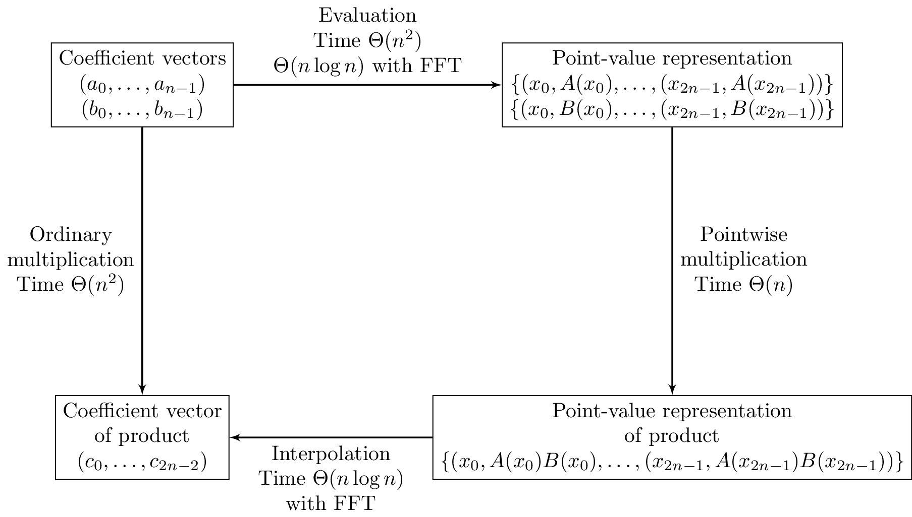
Outline of the approach to efficient polynomial multiplication using the fast Fourier transform.

In general, evaluating a polynomial A at a single point x takes Θ(n) operations, and since we have to evaluate 2n points, the evaluation step takes time Θ(n2). So it seems like we still aren’t doing any better than the ordinary multiplication algorithm.

The key point is that the evaluation step will take Θ(n2) operations if we just choose any old points x0,…,x2n−1. But for a particular choice of points, namely, the complex roots of unity, we’ll see how we can evaluate A on that set of points using only Θ(nlogn) operations, using the fast Fourier transform. It’ll also be possible to use the FFT to do the interpolation step, once we have the product of A and B in point-value form.

Complex Roots of Unity

A number z∈C is an nth root of unity if zn=1. The principal nth root of unity is ωn=e2πin. For n≥1, the n nth roots of unity are ω0n,ω1n,…,ωn−1n. For a bit of geometric intuition, the nth roots of unity form the vertices of a regular n-gon in the complex plane. We’ll use a few basic properties of complex roots of unity.

Lemma. (Cancellation lemma) For integers n≥0, k≥0, d>0, we have ωdkdn=ωkn.

Proof. ωdkdn=(e2πidn)dk=e2πikn=ωkn.

Corollary. (Halving lemma) If n>0 is even, and k>0, we have (ωkn)2=ωkn/2.

The proof essentially amounts to applying the cancellation lemma with d=2. What halving lemma means though, is that if n is even, then squaring each of the n complex nth roots of unity gives us exactly the n2 complex n2th roots of unity.

Note that squaring all of the nth roots of unity gives us each n2th root of unity twice, since (ωk+n/2n)2=ω2k+nn=ω2knωnn=(ωkn)2.

Lemma. (Summation lemma) If n≥1 and k is not divisible by n, then

n−1∑j=0(ωkn)j=0.

Proof. Using the formula for the sum of a geometric series,

n−1∑j=0(ωkn)j=(ωkn)n−1ωkn−1=(ωnn)k−1ωkn−1=1k−1ωkn−1=0.

Since k is not divisible by n, we know that ωkn≠1, so that the denominator is not zero.

The Discrete Fourier Transform for Polynomial Evaluation

Now we are ready to define the discrete Fourier transform, and see how it can be applied to the problem of evaluating a polynomial on the complex roots of unity.

Definition. Let a=(a0,…,an−1)∈Cn. The discrete Fourier transform of a is the vector DFTn(a)=(ˆa0,…,ˆan−1), where⁴

ˆak=n−1∑j=0aje2πikjn=n−1∑j=1ajωkjn0≤k≤n−1.

If you look closely, you can see that this definition is in fact exactly what we want. Let A(x)=a0+a1x+a2x2+⋯+an−1xn−1 be the polynomial whose coefficients are given by a. Then for 0≤k≤n−1, the polynomial A evaluated at the root of unity ωkn is exactly

A(ωkn)=n−1∑j=0aj(ωkn)j=ˆak.

Here, the n is really the 2n from previous sections, however we will simply use n to denote the length of the vector a when describing the DFT to simplify matters.

So far though, we still haven’t gained much, since applying this definition and directly computing the sum for each k takes Θ(n2) operations. This is where the fast Fourier transform comes in: this will allow us to compute DFTn(a) in time Θ(nlogn).

Fast Fourier Transform

The fast Fourier transform is an algorithm for computing the discrete Fourier transform of a sequence by using a divide-and-conquer approach.

As always, assume that n is a power of 2. Given a=(a0,…,an−1)∈Cn, we have the polynomial A(x), defined as above, which has n terms. We can also define two other polynomials, each with n2 terms, by taking the even and odd coefficients of A, respectively:

Ae(x)=a0+a2x+a4x2+⋯+an−2xn2−1,Ao(x)=a1+a3x+a5x2+⋯+an−1xn2−1.

Then, for any x∈C, we can evaluate A at x using the formula

A(x)=Ae(x2)+xAo(x2).

So the problem of evaluating A at ω0n,ω1n,…,ωn−1n reduces to performing the following steps:

1. Evaluate the two polynomials Ae and Ao of degree n2−1 at the points (ω0n)2,(ω1n)2,…,(ωn−1n)2.
2. Use the formula (∗) to combine the results from step 1.

By the halving lemma, we only actually need to evaluate Ae and Ao at n2 points, rather than at all n points. Thus, at each step, we divide the initial problem of size n into two subproblems of size n2.

Now that we have the general idea behind how the FFT works, we can look at some pseudocode.⁵

function Fast-Fourier-Transform(\(a\))

    \(n = a.\mathit{length}\)
    if \(n = 1\)
        return \(a\)

    \(a_e = (a_0, a_2, \dots, a_{n-2})\)
    \(a_o = (a_1, a_3, \dots, a_{n-1})\)

    \(y_e =\) Fast-Fourier-Transform(\(a_e\))
    \(y_o =\) Fast-Fourier-Transform(\(a_o\))

    \(\omega_n = e^{\frac{2\pi i}{n}}\)
    \(\omega = 1\)

    for \(k = 0\) to \(\frac{n}{2} - 1\)
        \(y_k = (y_e)_k + \omega(y_0)_k\)
        \(y_{k + \frac{n}{2}} = (y_e)_k - \omega(y_o)_k\)
        \(\omega = \omega\omega_n.\) // \(\omega = \omega_n^{k+1}\)

    \(y = (y_0,\dots, y_{n-1})\)
    return \(y\)

• function Fast-Fourier-Transform(a)
• • n=a.length
  • if n=1
    • return a
• • ae=(a0,a2,…,an−2)
  • ao=(a1,a3,…,an−1)
• • ye= Fast-Fourier-Transform(ae)
  • yo= Fast-Fourier-Transform(ao)
• • ωn=e2πin
  • ω=1
• • for k=0 to n2−1
    • yk=(ye)k+ω(y0)k
    • yk+n2=(ye)k−ω(yo)k
    • ω=ωωn. // ω=ωk+1n
• • y=(y0,…,yn−1)
  • return y

The pseudocode more or less follows the algorithmic structure outlined above. The main thing that we need to check is that the for loop actually combines the results using the correct formula. For k=0,1,…,n2−1, in the recursive calls we compute, by the cancellation lemma,

(ye)k=Ae(ωkn/2)=Ae(ω2kn),(yo)k=Ao(ωkn/2)=Ao(ω2kn).

In the for loop, for each k=0,…,n2−1, we compute

yk=Ae(ω2kn)+ωknAo(ω2kn)=A(ωkn).

We also compute

yk+n2=Ae(ωkn/2)−ωknAo(ωkn/2)=Ae(ω2kn)+ωk+n2nAo(ω2kn)=Ae(ω2k+nn)+ωk+n2nAo(ω2k+nn)=A(ωk+n2n).

Therefore yk=A(ωkn)=ˆak for all 0≤k≤n−1, and therefore this algorithm returns the correct result. Moreover, let T(n) denote the running time of Fast-Fourier-Transform(a) when a has length n. Since the algorithm makes two recursive calls on subproblems of size n2, and uses Θ(n) steps to combine the results, the overall running time of this algorithm is

T(n)=2T(n2)+Θ(n)=Θ(nlogn).

Inversion Formula and Interpolation via FFT

Now that, given the coefficients of a polynomial, we can evaluate it on the roots of unity by using the FFT, we want to perform the inverse operation, interpolating a polynomial from its values on the nth roots of unity, so that we can convert a polynomial from its point-value representation, back to its coefficient representation.

The first idea here will be to observe that DFTn:Cn→Cn is a linear map. This means that it can be written in terms of a matrix multiplication:

[111⋯11ωnω2n⋯ωn−1n⋮⋮⋮⋱⋮1ωn−1nω2(n−1)n⋯ω(n−1)2n][a0a1⋮an−1]=[ˆa0ˆa1⋮ˆan−1].

We can denote the matrix on the left-hand side of this equation by Mn(ωn). This matrix has a special name in linear algebra, and is called a Vandermonde matrix. To solve the problem of performing the reverse of the discrete Fourier transform, and convert from the point-value representation to the coefficient representation of a polynomial, we simply need to find the inverse of this matrix. It turns out that the structure of this particular matrix makes it particularly easy to invert.

Theorem. (Inversion formula) For n≥1, the matrix Mn(ωn) is invertible, and

Mn(ωn)−1=1nMn(ω−1n).

Proof. The (j,j′) entry of Mn(ωn) is equal to ωjj′n. Similarly, the (j,j′) entry of 1nMn(ω−1n) is 1nω−jj′n. Therefore, the (j,j′) entry of the product 1nMn(ω−1n)Mn(ωn) is equal to

1nn−1∑k=0ω−kjnωkj′n=1nn−1∑k=0ωk(j′−j)n.

If j′=j, then this sum equals n, and so the entire expression evaluates to 1. On the other hand, if j′≠j, then this sum equals 0, by the summation lemma. Therefore 1nMn(ω−1n)Mn(ωn)=In, the n×n identity matrix, and so Mn(ωn)−1=1nMn(ω−1n).

This key takeaway of this inversion formula is that it enables us to invert the discrete Fourier transform by using the exact same algorithm as the fast Fourier transform, but with ωn replaced with ω−1n, and then dividing the entire result by n. Therefore it is also possible to perform polynomial interpolation (from the complex roots of unity) in time Θ(nlogn).

Putting it all together, this demonstrates how it is possible to multiply two polynomials, by computing their values on the 2nth roots of unity, doing pointwise multiplication, and interpolating the result to obtain the coefficients of the product. All of this takes time Θ(nlogn), which is a significant improvement over the naive Θ(n2) algorithm.

References

[1] Cooley, J.W. and Tukey, J.W. 1965. An algorithm for the machine calculation of complex fourier series. Mathematics of computation. 19, 90 (1965), 297–301.
[2] Cormen, T.H., Leiserson, C.E., Rivest, R.L. and Stein, C. 2009. Introduction to algorithms, third edition. The MIT Press.
[3] Dasgupta, S., Papadimitriou, C.H. and Vazirani, U. 2008. Algorithms. McGraw-Hill, Inc.
For simplicity, we’ll assume that \(n\) is a power of 2.↩︎
This system of equations is defined using a Vandermonde matrix, which we’ll see in more detail later.↩︎
We use \(2n\) point-value pairs instead of just \(2n-1\), since if \(n\) is a power of 2, then so is \(2n\). This will be useful later.↩︎
If you’ve seen Fourier transforms before in the context of signal processing or other areas, you’ve probably seen it defined in terms of \(\omega_n^{-1}\) rather than \(\omega_n\). The form used here simplifies matters a bit for our specific application, and the math is almost the same either way.↩︎
Thanks to jQuery Pseudocode by David Stutz, for excellent pseudocode formatting script.↩︎